First Law of Thermodynamics

The review for the quiz for the beginning of the class on evaluating the graph and finding the mass of the water.

Prof Mason submerging the flask into ice water and warm water.  The syringe acts like a piston and displace a change in volume inside the syringe.

Our prediction of the work being done by the system shown that the syringe will move  upwards (increasing in volume).

The first law of thermodynamic on the left side, and the interpretation of the first law in the words for a 7 yr old to understand.

Examples of isothermal process:   a balloon losing air and the change of volume is the work done on the system.

A sample calculation from the lecture to find the change of volume using work = (delta)V*p and the conversion of units. 

The derivation of a function in terms of mass and velocity.

Using a cube, we find the function of pressure in terms of volume.

Using relation of pressure we find in the above picture, we find the function of temperature in terms of kinetic energy.

We further examined the isothermal process by evaluating the inernal energy, and the adiabatic process from work done.

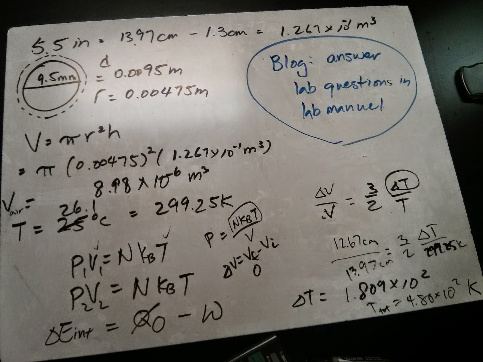
The calculation of the change of temperature inside the fire syringe.  The change of volume from the work done on the system causes the temperature to go up high rapidly due to the inverse relationship of volume and pressure. 

Homework:

Thermal Properties of Matter cont.

The prediction of the hot aluminum can rapidly implode when submerged into ice water sealing off the opening.  The can immediately shrunk the volume.

The aluminum can took in the volume of the water as the temperature drops, instead of shrinking the volume of itself.

The seven units of pressure and the conversion of atm to Pa.

Prediction graph of the relationship of pressure versus volume.  The graph predicts an inverse relationship decaying as volume increases.

The actual experiment using lab instruments and the line fit using y=1/ax+b.  The fit of the curve is inverse with the adjustment of b shifting the graph to where the data line is.

The prediction of the pressure versus temperature graph.

The data for initial pressure and temperature before the start of the experimentation.

Data from the experiment showing a linear relationship instead of the curved relationship as predicted in the previous photo.

The further examination of the Boltzmann's constant, the R constant, and Avogadro's constant.

Sample calculation from the lecture notes

The increase of volume when pressure of the air was vacuumed away.  The balloon was dramatically increasing in size.

Prof Mason released the pressure and the balloon goes back in it's original volume.

Our prediction of the balloon and marshmellow in the vacuum pressure chamber.

Sample calculation from the lecture notes.

Heat (cont.) and Thermal Properties of Matter

The atomic level of the crystal lattice of a substance in solid state going through an increase of energy, therefore expanding the distance of the bonding between each atom.

An short explanation of the binding expansion.  This also concurs with the prediction that the heated ring will have a greater radius. 

Thermal expansion diagram and the dependent variables of the expansion.

Prof Mason demonstrating the expansion when the brass and Invar under goes thermal expansion.

The prediction concurs that the rod curves toward the Invar side because of the Invar has a higher coefficient of the expansion.

Prof Mason heading the rod on the brass side.

Prof Mason expose the rod into water and ice.

Black is the prediction of the heating Invar side.  Green is the prediction of the heating brass side.  Blue is the prediction of the rod going into ice water.  All prediction were right!

The set up of aluminum rod with steam under going thermal expansion to the heat of the steam.

The aluminum rod going through thermal expansion when exposed to steam.

The actual board calculation of the thermal expansion of the rod.  The angle of the sensor and the radius gives us the arc length of the sector.  The sector is the expansion of the rod (delta)L.  The calculated length from the experimental value is 19 x 10^-6 (C^-1)

**(The uncertainty of the length will be at the bottom of this page)

Graph of the ice water going through change of state and reaching boiling point.  This picture was taken immediately when boiling point was reach.  In the picture, the boiling point was actually 98 decree C, not the theoretical 100 decree C.

This picture was taking after certain amount of time after the heat was discontinued.  The graph, however, was fitted by LoggerPro and displayed the slope of the line.

Calculation of the calorimetry; finding the mass needed for the change of the temperature.

Calculation of finding the "lucky" constant using Q = mc(delta)T;  Also, a brief explanation of the error that involves with official lab report (systematic error and random error).

The 5 state of matters on the top of the board.  A calculation of the change of state given energy.  However, this energy (215kJ) never exceeded the 263860 J that's needed to completely melt the ice, therefore the T-final is 0 degree C.

Activity of the mass of water that can be poured onto the 255g of ice without the ice melting.

Here's Daniel blowing in air for the displacement of the water level.

By measuring the displacement of the water level, we can therefore find the total volume of the straw.  Using the density of the water, we can find the total pressure of the air being blown into the straw by Daniel.

Propagating the uncertainty for the change of the length of the aluminum rod:

The uncertainty is 1.2x10^-5 (C^-1).  

Which our final answer should be  19 x 10^-6 (C^-1) +/- 1.2x10^-5 (C^-1).  The theoretical value were within the uncertainty of the experiment.

Temperature and Heat

Graph of the thermal equilibrium of 2 cups of tap water with different temperature.  The temperature displaces the final temperature.  Time of the photo was taken immediately when thermal equilibrium was reach to avoid the lost of energy to surrounding.

Calculation of the final temperature using Q = mc(delta)T  

By setting the Q = Q, we can find Tf because of thermal equilibrium occurs at final temperature.

The experiment of specific heat using temperature probe with an aluminium can as a heat conductor in water, and possibilities of the high experimental error.  Experimental specific heat for aluminum yield to be 16.3.  Intuitively we know that 16 must be an error when compare to 4.186 of water specific heat.  The propagation of uncertainty will be displayed at the bottom.

Graph of the aluminium can as a heat conductor submerged in water and the data.  The disturbance of the graph was due to the stiring and handling of the experiment equipment.

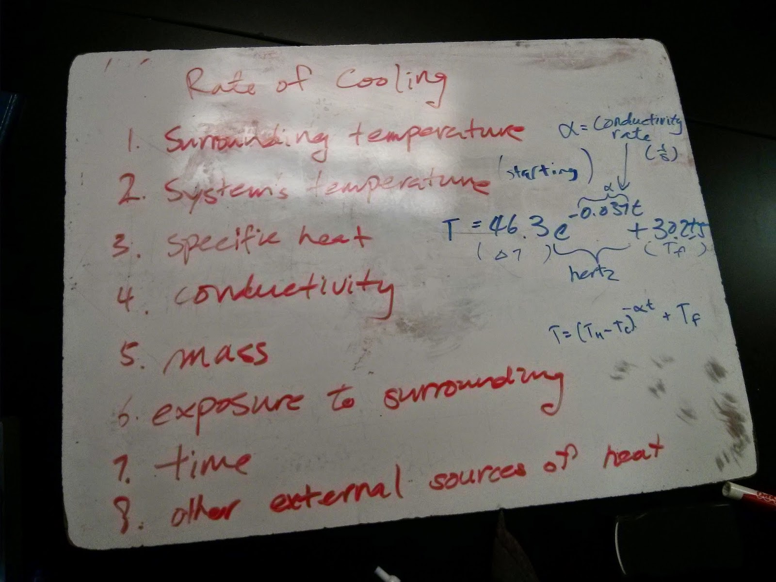
The group discussion of the possibilities of factors that can alter the rate of cooling variables.  In blue: the relationship of heat transfer and the meaning of each unit explained in lecture.

The relationship of dependent and independent variables that determinate the heat and the proportionality.

Group activity of Aluminium and Copper rod in contact for heat transfer and (delta)T.  Our side of the room were to calculate the heat transfer for the blue rod (aluminum).  Surprisingly, the class discovered that heat transfered by both Copper and Aluminum were the same, 67.7 degree C.

The experimental value of the heat transfer into water with respect to time.  The slope in the graph (fitted by the program) is the rate (ratio) of energy and temperature.

Calculation of the heat transfer into water activity to find the specific heat (c). 

Class activity of the uncertainty to demonstrate the acceptable way of scientific experiment and acceptable interpretation of the values.

Summary:
Any thing that comes in contact with another mass that has a different temperature will cause heat to transfer from high to low.  The system will eventually come in equilibrium thermally unless another source of heat would be introduced.  The lecture also covered thermal expansions, heat transfer, heat capacity calculations.



Uncertainty of the heat transfer activity:

Using the equation Q = mc(delta)T , we can relate the mass, specific heat, and temperature difference in a relation.  In the activity, this equation is also used to propagate the uncertainty of the equipment used during the experiment. 

The actual calculations:

In conclusion to the Aluminium can experiment, the final result of the experimental specific heat should be 16.8 +/- 28.  The result were withing the uncertainty despite the theoretical value was smaller by 4 factors.  The high experimental value could be a combination of systematic error (i.e. equipment un-calibrated, digital scare not tared before usage, the Mason-estimation on the initial temperature and the Mason-estimation on the mass of the aluminium can.)